Routing

Often when creating a design, you need to connect geometries together with wires or waveguides. To help with that, PHIDL has the phidl.routing (pr) module, which can flexibly and quickly create routes between ports.

Simple quadrilateral routes

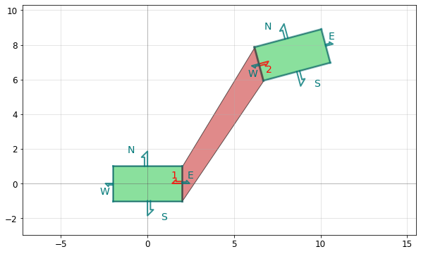
In general, a route is a polygon used to connect two ports. Simple routes are easy to create using pr.route_quad(). This function returns a quadrilateral route that directly connects two ports, as shown in this example:

from phidl import Device, quickplot as qp
import phidl.geometry as pg
import phidl.routing as pr

# Use pg.compass() to make 2 boxes with North/South/East/West ports
D = Device()
c1 = D << pg.compass()
c2 = D << pg.compass().move([10,5]).rotate(15)

# Connect the East port of one box to the West port of the other
R = pr.route_quad(c1.ports['E'], c2.ports['W'],
                  width1 = None, width2 = None,  # width = None means use Port width
                  layer = 2)
qp([R,D])

Automatic manhattan routing

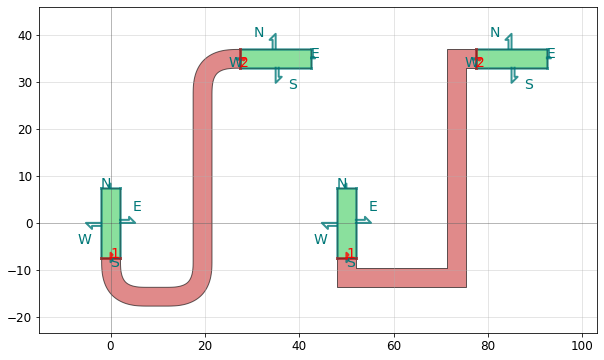
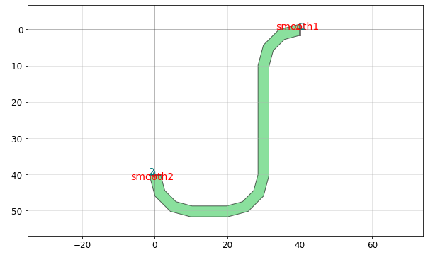
In many cases, we need to draw wires or waveguides between two objects, and we’d prefer not to have to hand-calculate all the points. In these instances, we can use the automatic routing functions pr.route_smooth() and pr.route_sharp().

These functions allow you to route along a Path, and come with built-in options that let you control the shape of the path and how to extrude it. If you don’t need detailed control over the path your route takes, you can let these functions create an automatic manhattan route by leaving the default path_type='manhattan'. Just make sure the ports you’re to routing between face parallel or orthogonal directions.

from phidl import Device, quickplot as qp
import phidl.geometry as pg
import phidl.routing as pr

# Use pg.compass() to make 4 boxes with North/South/East/West ports
D = Device()
smooth1 = D << pg.compass([4,15])
smooth2 = D << pg.compass([15,4]).move([35,35])
sharp1 = D << pg.compass([4,15]).movex(50)
sharp2 = D << pg.compass([15,4]).move([35,35]).movex(50)

# Connect the South port of one box to the West port of the other
R1 = pr.route_smooth(smooth1.ports['S'], smooth2.ports['W'], radius=8, layer = 2)
R2 = pr.route_sharp(  sharp1.ports['S'],  sharp2.ports['W'], layer = 2)

qp([D, R1, R2])

Customized widths / cross-sections

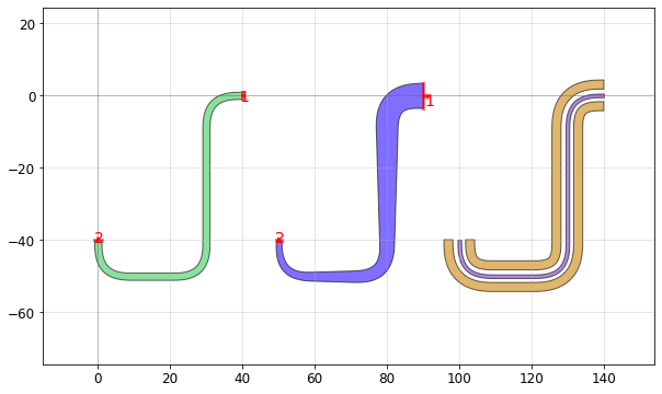
By default, route functions such as route_sharp() and route_smooth() will connect one port to another with polygonal paths that are as wide as the ports are. However, you can override this by setting the width parameter in the same way as extrude():

• If set to a single number (e.g. width=1.7): makes a fixed-width extrusion

• If set to a 2-element array (e.g. width=[1.8,2.5]): makes an extrusion whose width varies linearly from width[0] to width[1]

• If set to a CrossSection: uses the CrossSection parameters for extrusion

from phidl import CrossSection
import phidl.routing as pr

# Create input ports
port1 = D.add_port(name='smooth1', midpoint=(40,  0), width=5, orientation=180)
port2 = D.add_port(name='smooth2', midpoint=(0, -40), width=5, orientation=270)

# (left) Setting width to a constant
D1 = pr.route_smooth(port1, port2, width = 2, radius=10, layer = 0)

# (middle) Setting width to a 2-element list to linearly vary the width
D2 = pr.route_smooth(port1, port2, width = [7, 1.5], radius=10, layer = 1)

# (right) Setting width to a CrossSection
X = CrossSection()
X.add(width=1, layer=4)
X.add(width=2.5, offset =  3, layer = 5)
X.add(width=2.5, offset = -3, layer = 5)
D3 = pr.route_smooth(port1, port2, width = X, radius=10)

qp([D1, D2.movex(50), D3.movex(100)])

Details of operation

The route_smooth() function works in three steps:

1. It calculates a waypoint Path using a waypoint path function – such as pr.path_manhattan() – set by the path_type.

2. It smooths out the waypoint Path using pp.smooth().

3. It extrudes the Path to create the route geometry.

The route_sharp() function works similarly, but it omits step 2 to create sharp bends. The extra smoothing makes route_smooth() particularly useful for photonic / microwave waveguides, whereas route_sharp() is typically more useful for electrical wiring.

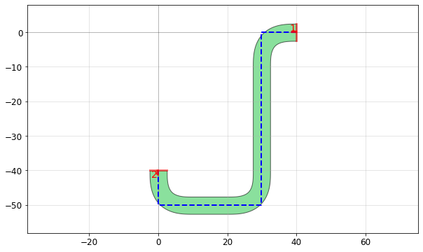
To illustrate how these functions work, let’s look at how you could manually implement a similar behaviour to route_smooth(path_type='manhattan'):

from phidl import CrossSection
import phidl.path as pp

D = Device()
port1 = D.add_port(name=1, midpoint=(40,0), width=5, orientation=180)
port2 = D.add_port(name=2, midpoint=(0, -40), width=5, orientation=270)

# Step 1: Calculate waypoint path
route_path = pr.path_manhattan(port1, port2, radius=10)
# Step 2: Smooth waypoint path
smoothed_path = pp.smooth(route_path, radius=10, use_eff=True)
# Step 3: Extrude path
D.add_ref(smoothed_path.extrude(width=5, layer=0))

qp([route_path,D])

We can even customize the bends produced by pr.route_smooth() using the smooth_options, which are passed to pp.smooth(), such as controlling the corner-smoothing function or changing the number of points that will be rendered:

D = Device()
port1 = D.add_port(name='smooth1', midpoint=(40,0), width=3, orientation=180)
port2 = D.add_port(name='smooth2', midpoint=(0, -40), width=3, orientation=270)
D.add_ref(pr.route_smooth(port1, port2, radius=10, smooth_options={'corner_fun': pp.arc, 'num_pts': 16}))
qp(D)

Customizing route paths

Avoiding obstacles

Sometimes, automatic routes will run into obstacles in your layout, like this:

import phidl.geometry as pg

D = Device()
Obstacle = D.add_ref(pg.rectangle(size=(30,15), layer=1)).move((10, -25))

port1 = D.add_port(name=1, midpoint=(40,0), width=5, orientation=180)
port2 = D.add_port(name=2, midpoint=(0, -40), width=5, orientation=270)

D.add_ref(pr.route_smooth(port1, port2, radius=10, path_type='manhattan'))
qp(D)

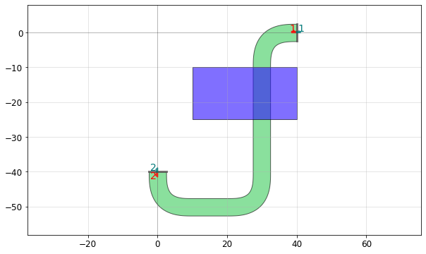
Example 1: Custom ``J`` paths. To avoid the other device, we need to customize the path our route takse. Luckily, PHIDL provides several waypoint path functions to help us do that quickly. Each of these waypoint path functions has a name of the form pr.path_*** (e.g. pr.path_L()), and generates a particular path type with its own shape. All the available path types are described in detail below and in the Geometry Reference. In this case, we want to connect two orthogonal ports, but the ports are positioned such that we can’t connect them with a single 90-degree turn. A J-shaped path with four line segments and three turns is perfect for this problem. We can tell route_smooth to use pr.path_J() as its waypoint path function via the argument path_type='J'.

D = Device()
Obstacle = D.add_ref(pg.rectangle(size=(30,15), layer=1))
Obstacle.move((10, -25))
port1 = D.add_port(name=1, midpoint=(40,0), width=5, orientation=180)
port2 = D.add_port(name=2, midpoint=(0, -40), width=5, orientation=270)

D.add_ref(pr.route_smooth(port1, port2, radius=10, path_type='J', length1=60, length2=20))
qp(D)

For ease of use, the waypoint path functions are parameterized in terms of relative distances from ports. Above, we had to define the keyword arguments length1 and length2, which are passed to pr.route_J() for the waypoint path calculation. These arguments length1 and length2 define the lengths of the line segments that exit port1 and port2 respectively (i.e. the first and last sements in the path). Once those first and last segments are set, path_J() completes the waypoint path with two more 90-degree turns. Note that just knowing length1 and length2, along with the port positions and orientations, is enough to completely determine the waypoint path.

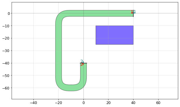
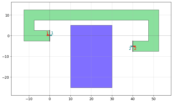
Example 2: Custom ``C`` paths. Now consider this routing problem:

D = Device()
Obstacle = D.add_ref(pg.rectangle(size=(20,30),layer=1))
Obstacle.move((10, -25))
port1 = D.add_port(name=1, midpoint=(0,0), width=5, orientation=180)
port2 = D.add_port(name=2, midpoint=(40, -5), width=5, orientation=0)

D.add_ref(pr.route_sharp(port1, port2, path_type='manhattan'))
qp(D)

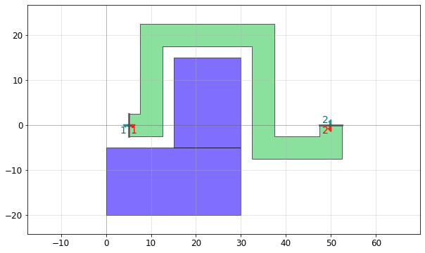
In this case, we want a C path. C paths have three parameters we need to define: + length1 and length2, which are the lengths of the segments that exit port1 and port2 (similar to the J path), as well as + left1, which is the length of the segment that turns left from port1.

In this case, we would actually prefer that the path turns right after it comes out of port1, so that our route avoids the other device. To make that happen, we can just set left1<0:

D = Device()
Obstacle = D.add_ref(pg.rectangle(size=(20,30),layer=1))
Obstacle.move((10, -25))
port1 = D.add_port(name=1, midpoint=(0,0), width=5, orientation=180)
port2 = D.add_port(name=2, midpoint=(40, -5), width=5, orientation=0)

D.add_ref(pr.route_sharp(port1, port2, path_type='C', length1=10, length2=10, left1=-10))
qp(D)

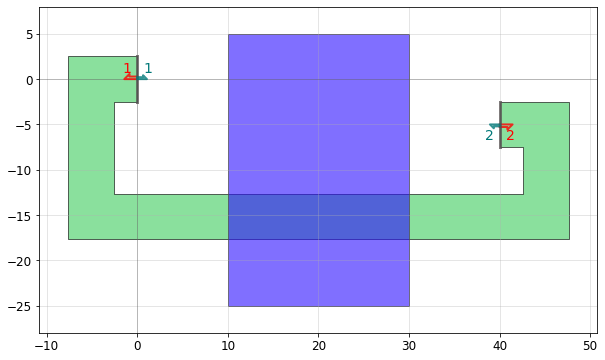
Example 3: Custom ``manual`` paths. For even more complex route problems, we can use path_type='manual' to create a route along an arbitrary path. In the example below, we use a manual path to route our way out of a sticky situation:

D = Device()
Obstacle = D.add_ref(pg.rectangle(size=(30,15),layer=1)).move((0, -20))
Obstacle2 = D.add_ref(pg.rectangle(size=(15,20), layer=1))
Obstacle2.xmax,Obstacle2.ymin = Obstacle.xmax, Obstacle.ymax

port1 = D.add_port(name=1, midpoint=(5,  0), width=5, orientation=0)
port2 = D.add_port(name=2, midpoint=(50, 0), width=5, orientation=270)

manual_path = [ port1.midpoint,
                (Obstacle2.xmin-5, port1.y),
                (Obstacle2.xmin-5, Obstacle2.ymax+5),
                (Obstacle2.xmax+5, Obstacle2.ymax+5),
                (Obstacle2.xmax+5, port2.y-5),
                (port2.x, port2.y-5),
                port2.midpoint ]

D.add_ref(pr.route_sharp(port1, port2, path_type='manual', manual_path=manual_path))
qp(D)

Note that to manually route between two ports, the first and last points in the manual_path should be the midpoints of the ports.

List of routing path types

PHIDL provides the following waypoint path types for routing:

Path type	Routing style	Segments	Useful for …	Parameters
manhattan	Manhattan	1-5	parallel or orthogonal ports.	radius
straight	Manhattan	1	ports that point directly at each other.	–
L	Manhattan	2	orthogonal ports that can be connected with one turn.	–
U	Manhattan	3	parallel ports that face each other or same direction.	length1
J	Manhattan	4	orthogonal ports that can’t be connected with just one turn.	length1, length2
C	Manhattan	5	parallel ports that face apart.	length1, length2, left1
V	Free	2	ports at odd angles that face a common intersection point.	–
Z	Free	3	ports at odd angles.	length1, length2
manual	Free	–	fully custom paths.	manual_path

For more details on each path type, you can also look at the API Documentation or the Geometry Reference.

The path types can be classified by their routing style. Manhattan style routing uses only 90-degree turns, and thus requires that you route between ports that are orthogonal or parallel (note that the ports don’t neccearrily have to point horizontally or vertically, though). For routing between ports at odd angles, you can use path types with a free routing style instead.

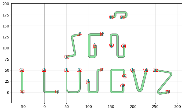
Most path types are named after letters that they resemble to help you remember them. However, as you’ll see in the examples below, some of the more complicated paths can take a variety of shapes. One good way to identify which manhattan-style route type you need is to count the number of line segments and consult the above table.

D = Device()

#straight path
port1 = D.add_port(name='S1', midpoint=(-50, 0), width=4, orientation=90)
port2 = D.add_port(name='S2', midpoint=(-50, 50), width=4, orientation=270)
D.add_ref(pr.route_smooth(port1, port2, path_type='straight'))
#L path
port1 = D.add_port(name='L1', midpoint=(30,0), width=4, orientation=180)
port2 = D.add_port(name='L2', midpoint=(0, 50), width=4, orientation=270)
D.add_ref(pr.route_smooth(port1, port2,  path_type='L'))
#U path
port1 = D.add_port(name='U1', midpoint=(50, 50), width=2, orientation=270)
port2 = D.add_port(name='U2', midpoint=(80,50), width=4, orientation=270)
D.add_ref(pr.route_smooth(port1, port2,  radius=10, path_type='U', length1=50))
port1 = D.add_port(name='U3', midpoint=(50, 80), width=4, orientation=10)
port2 = D.add_port(name='U4', midpoint=(80, 130), width=4, orientation=190)
D.add_ref(pr.route_smooth(port1, port2,  path_type='U', length1=20))
#J path
port1 = D.add_port(name='J1', midpoint=(100, 25), width=4, orientation=270)
port2 = D.add_port(name='J2', midpoint=(130, 50), width=4,  orientation=180)
D.add_ref(pr.route_smooth(port1, port2,  path_type='J', length1=25, length2=10))
port1 = D.add_port(name='J3', midpoint=(115, 105), width=5, orientation=270)
port2 = D.add_port(name='J4', midpoint=(131, 130), width=5,  orientation=180)
D.add_ref(pr.route_smooth(port1, port2, path_type='J', length1=25, length2=30))
#C path
port1 = D.add_port(name='C1', midpoint=(180, 35), width=4, orientation=90)
port2 = D.add_port(name='C2', midpoint=(178, 15), width=4, orientation=270)
D.add_ref(pr.route_smooth(port1, port2, path_type='C', length1=15, left1=30, length2=15))
port1 = D.add_port(name='C3', midpoint=(150, 105), width=4, orientation=90)
port2 = D.add_port(name='C4', midpoint=(180, 105), width=4, orientation=270)
D.add_ref(pr.route_smooth(port1, port2, path_type='C', length1=25, left1=-15, length2=25))
port1 = D.add_port(name='C5', midpoint=(150, 170), width=4, orientation=0)
port2 = D.add_port(name='C6', midpoint=(175, 170), width=4, orientation=0)
D.add_ref(pr.route_smooth(port1, port2, path_type='C', length1=10, left1=10, length2=10, radius=4))
#V path
port1 = D.add_port(name='V1', midpoint=(200,50), width=5, orientation=284)
port2 = D.add_port(name='V2', midpoint=(230, 50), width=5, orientation=270-14)
D.add_ref(pr.route_smooth(port1, port2, path_type='V'))
#Z path
port1 = D.add_port(name='Z1', midpoint=(280,0), width=4, orientation=190)
port2 = D.add_port(name='Z2', midpoint=(250, 50), width=3, orientation=-10)
D.add_ref(pr.route_smooth(port1, port2, path_type='Z', length1=30, length2=40))


qp(D)

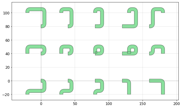
The manhattan path type is bending-radius aware and can produce any route neccessary to connect two ports, as long as they are orthogonal or parallel.

import numpy as np
set_quickplot_options(show_ports=False, show_subports=False)

D = Device()
pitch = 40
test_range=20
x_centers = np.arange(5)*pitch
y_centers = np.arange(3)*pitch
xoffset = np.linspace(-1*test_range, test_range, 5)
yoffset = np.linspace(-1*test_range, test_range, 3)
for xidx, x0 in enumerate(x_centers):
    for yidx, y0 in enumerate(y_centers):
        name = '{}{}'.format(xidx, yidx)
        port1 = D.add_port(name=name+'1', midpoint=(x0, y0), width=5, orientation=0)
        port2 = D.add_port(name=name+'2', midpoint=(x0+xoffset[xidx], y0+yoffset[yidx]),
                           width=5,  orientation=90)
        D.add_ref(pr.route_smooth(port1, port2, route_type='manhattan'))
qp(D)

Simple XY wiring

Often one requires simple wiring between two existing objects with Ports. For this purpose, you can use the route_xy() function. It allows a simple string to specify the path the wiring will take. So the argument directions = 'yxy' means “go 1 part in the Y direction, 1 part in the X direction, then 1 more part in the X direction” with the understanding that 1 part X = (total X distance from port1 to port2)/(total number of ‘x’ in the directions)

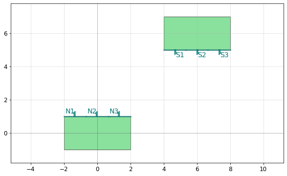
As an example, say we have two objects with multiple ports, and we want to route multiple wires between them without overlapping

from phidl import Device, quickplot as qp
import phidl.routing as pr
import phidl.geometry as pg

# Create boxes with multiple North/South ports
D = Device()
c1 = D.add_ref( pg.compass_multi(ports={'N':3}) )
c2 = D.add_ref( pg.compass_multi(ports={'S':3}) ).move([6,6])

qp(D)

We can then route_xy() between them and use different directions arguments to prevent them from overlapping:

D.add_ref( pr.route_xy(port1 = c1.ports['N1'], port2 = c2.ports['S1'],
    directions = 'yyyxy', width = 0.1, layer = 2) )
D.add_ref( pr.route_xy(port1 = c1.ports['N2'], port2 = c2.ports['S2'],
    directions = 'yyxy',  width = 0.2, layer = 2) )
D.add_ref( pr.route_xy(port1 = c1.ports['N3'], port2 = c2.ports['S3'],
    directions = 'yxy',   width = 0.4, layer = 2) )

qp(D)

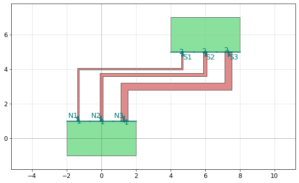
• In the first case, when directions = 'yyyxy': The route traveled up 3/4 of the total Y distance, then the full x distance, then the remaining 1/4 of the y distance (there are 4 y characters and only 1 x character)

• In the second case, when directions = 'yyxy': The route traveled up 2/3 of the total Y distance, then the full x distance, then the remaining 1/3 of the y distance

• In the third case, when directions = 'yxy': The route traveled up 1/2 of the total Y distance, then the full x distance, then the remaining 1/2 of the y distance